教程：通过 SQL 机器学习在 R 中创建预测模型

Applies to: SQL Server 2016 (13.x) and later Azure SQL Managed Instance

本文将指导如何进行以下操作：

In part one, you learned how to restore the sample database.

In part two, you learned how to load the data from a database into a Python data frame and prepare the data in R.

In part four, you'll learn how to store the model in a database, and then create stored procedures from the Python scripts you developed in parts two and three. 存储过程将在服务器上运行，以便基于新数据进行预测。

Prerequisites

Part three of this tutorial series assumes you have fulfilled the prerequisites of part one, and completed the steps in part two.

训练两个模型

若要找出滑雪器具租赁数据的最佳模型，请创建两个不同的模型（线性回归和决策树），看哪个模型做出的预测更准确。 你将使用在本系列的第一部分创建的数据帧 rentaldata。

#First, split the dataset into two different sets:
# one for training the model and the other for validating it
train_data = rentaldata[rentaldata$Year < 2015,];
test_data  = rentaldata[rentaldata$Year == 2015,];


#Use the RentalCount column to check the quality of the prediction against actual values
actual_counts <- test_data$RentalCount;

#Model 1: Use lm to create a linear regression model, trained with the training data set
model_lm <- lm(RentalCount ~  Month + Day + WeekDay + Snow + Holiday, data = train_data);

#Model 2: Use rpart to create a decision tree model, trained with the training data set
library(rpart);
model_rpart  <- rpart(RentalCount ~ Month + Day + WeekDay + Snow + Holiday, data = train_data);

通过这两个模型进行预测

使用预测函数通过每个已训练的模型预测租赁计数。

#Use both models to make predictions using the test data set.
predict_lm <- predict(model_lm, test_data)
predict_lm <- data.frame(RentalCount_Pred = predict_lm, RentalCount = test_data$RentalCount, 
                         Year = test_data$Year, Month = test_data$Month,
                         Day = test_data$Day, Weekday = test_data$WeekDay,
                         Snow = test_data$Snow, Holiday = test_data$Holiday)

predict_rpart  <- predict(model_rpart,  test_data)
predict_rpart <- data.frame(RentalCount_Pred = predict_rpart, RentalCount = test_data$RentalCount, 
                         Year = test_data$Year, Month = test_data$Month,
                         Day = test_data$Day, Weekday = test_data$WeekDay,
                         Snow = test_data$Snow, Holiday = test_data$Holiday)

#To verify it worked, look at the top rows of the two prediction data sets.
head(predict_lm);
head(predict_rpart);

结果集如下。

    RentalCount_Pred  RentalCount  Month  Day  WeekDay  Snow  Holiday
1         27.45858          42       2     11     4      0       0
2        387.29344         360       3     29     1      0       0
3         16.37349          20       4     22     4      0       0
4         31.07058          42       3      6     6      0       0
5        463.97263         405       2     28     7      1       0
6        102.21695          38       1     12     2      1       0
    RentalCount_Pred  RentalCount  Month  Day  WeekDay  Snow  Holiday
1          40.0000          42       2     11     4      0       0
2         332.5714         360       3     29     1      0       0
3          27.7500          20       4     22     4      0       0
4          34.2500          42       3      6     6      0       0
5         645.7059         405       2     28     7      1       0
6          40.0000          38       1     12     2      1       0

比较结果

现在，你想了解哪个模型提供最佳预测。 一种快速简便的方法是使用基本绘图函数来查看训练数据中实际值与预测值之间的差异。

#Use the plotting functionality in R to visualize the results from the predictions
par(mfrow = c(1, 1));
plot(predict_lm$RentalCount_Pred - predict_lm$RentalCount, main = "Difference between actual and predicted. lm")
plot(predict_rpart$RentalCount_Pred  - predict_rpart$RentalCount,  main = "Difference between actual and predicted. rpart")

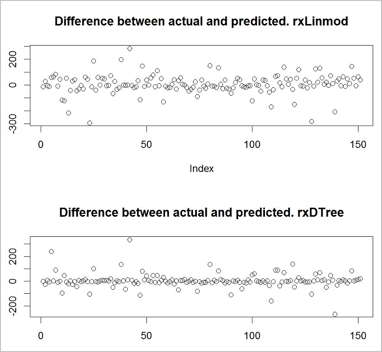
看起来决策树模型是两个模型中更准确的。

清理资源

如果不打算继续学习本教程，请删除 TutorialDB 数据库。

Next steps

在此教程系列的第三部分中，你已了解如何执行以下操作：

• 训练两个机器学习模型
• 通过这两个模型进行预测
• 比较结果以选择最准确的模型

若要部署已创建的机器学习模型，请按照本系列教程的第四部分进行操作：