チュートリアル:SQL 機械学習を使用して R で予測モデルを作成する

Applies to: SQL Server 2016 (13.x) and later Azure SQL Managed Instance

この記事では、次の方法について学習します。

In part one, you learned how to restore the sample database.

In part two, you learned how to load the data from a database into a Python data frame and prepare the data in R.

In part four, you'll learn how to store the model in a database, and then create stored procedures from the Python scripts you developed in parts two and three. ストアド プロシージャは、新しいデータに基づいて予測を行うためにサーバーで実行されます。

Prerequisites

Part three of this tutorial series assumes you have fulfilled the prerequisites of part one, and completed the steps in part two.

2 つのモデルをトレーニングする

スキー レンタル データに最適なモデルを見つけるために、2 つの異なるモデル (線形回帰とデシジョン ツリー) を作成し、どちらの予測がより正確であるかを調べます。 このシリーズのパート 1 で作成したデータ フレーム rentaldata を使用します。

#First, split the dataset into two different sets:
# one for training the model and the other for validating it
train_data = rentaldata[rentaldata$Year < 2015,];
test_data  = rentaldata[rentaldata$Year == 2015,];


#Use the RentalCount column to check the quality of the prediction against actual values
actual_counts <- test_data$RentalCount;

#Model 1: Use lm to create a linear regression model, trained with the training data set
model_lm <- lm(RentalCount ~  Month + Day + WeekDay + Snow + Holiday, data = train_data);

#Model 2: Use rpart to create a decision tree model, trained with the training data set
library(rpart);
model_rpart  <- rpart(RentalCount ~ Month + Day + WeekDay + Snow + Holiday, data = train_data);

両方のモデルで予測を行う

予測関数を使用し、トレーニング済みの各モデルを使ってレンタル数を予測します。

#Use both models to make predictions using the test data set.
predict_lm <- predict(model_lm, test_data)
predict_lm <- data.frame(RentalCount_Pred = predict_lm, RentalCount = test_data$RentalCount, 
                         Year = test_data$Year, Month = test_data$Month,
                         Day = test_data$Day, Weekday = test_data$WeekDay,
                         Snow = test_data$Snow, Holiday = test_data$Holiday)

predict_rpart  <- predict(model_rpart,  test_data)
predict_rpart <- data.frame(RentalCount_Pred = predict_rpart, RentalCount = test_data$RentalCount, 
                         Year = test_data$Year, Month = test_data$Month,
                         Day = test_data$Day, Weekday = test_data$WeekDay,
                         Snow = test_data$Snow, Holiday = test_data$Holiday)

#To verify it worked, look at the top rows of the two prediction data sets.
head(predict_lm);
head(predict_rpart);

結果セットは次のとおりです。

    RentalCount_Pred  RentalCount  Month  Day  WeekDay  Snow  Holiday
1         27.45858          42       2     11     4      0       0
2        387.29344         360       3     29     1      0       0
3         16.37349          20       4     22     4      0       0
4         31.07058          42       3      6     6      0       0
5        463.97263         405       2     28     7      1       0
6        102.21695          38       1     12     2      1       0
    RentalCount_Pred  RentalCount  Month  Day  WeekDay  Snow  Holiday
1          40.0000          42       2     11     4      0       0
2         332.5714         360       3     29     1      0       0
3          27.7500          20       4     22     4      0       0
4          34.2500          42       3      6     6      0       0
5         645.7059         405       2     28     7      1       0
6          40.0000          38       1     12     2      1       0

結果を比較する

次に、どちらのモデルで最善の予測が得られるかを調べます。 これを行うための迅速で簡単な方法は、基本的なプロット関数を使用して、トレーニング データの実際の値と予測値の差を表示することです。

#Use the plotting functionality in R to visualize the results from the predictions
par(mfrow = c(1, 1));
plot(predict_lm$RentalCount_Pred - predict_lm$RentalCount, main = "Difference between actual and predicted. lm")
plot(predict_rpart$RentalCount_Pred  - predict_rpart$RentalCount,  main = "Difference between actual and predicted. rpart")

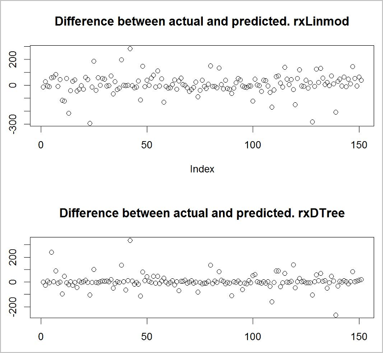
2 つのモデルのうち、デシジョン ツリー モデルの方がより正確であるように見えます。

リソースをクリーンアップする

このチュートリアルを続行しない場合は、TutorialDB データベースを削除してください。

Next steps

このチュートリアル シリーズのパート 3 で学習した内容は次のとおりです。

• 2 つの機械学習モデルをトレーニングする
• 両方のモデルで予測を行う
• 結果を比較して最も正確なモデルを選択する

作成した機械学習モデルをデプロイするには、このチュートリアル シリーズのパート 4 の手順に従います。