Configure relationships

When your model comprises more than one table, you need to ensure that appropriate relationships exist between the tables. Relationships propagate filters applied on one model table to a different model table. They continue to propagate so long as there's a relationship path to follow, which can involve propagation to multiple tables.

For example, when a visual filters the Year column of the Date table, a relationship to the Sales table automatically filters that table so that rows representing sales for that year are summarized. For report authors, this is normal and expected behavior.

Here's an animated example that shows how relationships propagate filters to other tables.

Configure data load options

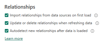
Before you apply your Power Query queries to load data to your model, you should first inspect the Power BI Desktop Data load options and adjust them when necessary.

Specifically, you might want to enable or disable relationship settings. When enabled, these settings can import relationships detected in source data, update or delete relationships when refreshing data, and autodetect new relationships.

When relationships aren't automatically created, you can create them in the Manage relationships window, or by switching to Model view.

Sometimes, a table doesn't need a relationship to another model table, which is known as a disconnected table. A disconnected table is useful when you want to support a what-if scenario or field parameters. Both scenarios are described later in this module.

Columns

Each relationship has a single "from" column and a single "to" column. It's important that the data types for these columns are the same (or equivalent) and that they contain matching values.

You should give consideration the relationships your model needs when defining the table structures in Power Query. To support the one-side of a relationship (described next), you must ensure that column contains unique values. Further, if your data source has a multi-column key, you need to transform the data to produce single-column keys for the related tables. If the related column data types don't match, you can adjust the data types with Power Query.

Understand cardinality

Every relationship has a cardinality type, which is either:

• One-to-many (1:*)
• Many-to-one (*:1)
• One-to-one (1:1)
• Many-to-many (*:*)

When Power BI Desktop automatically creates a relationship, it determines the cardinality based on the values already loaded into the columns. Sometimes, it might not set it correctly (because the table is yet to be loaded with rows of data), so you need to update the setting.

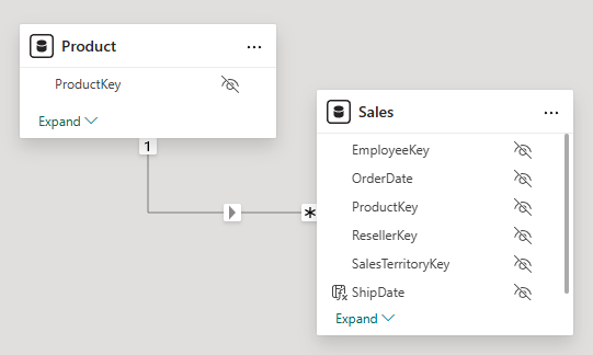
The One-to-many and Many-to-one relationships are essentially the same, just in different directions. They're the most commonly set cardinality types, typically supporting relationships between dimension tables (the "one" side) and fact tables (the "many" side) in a star schema design.

For example, the ProductKey column in the Product table has a one-to-many relationship with the ProductKey column in the Sales table.

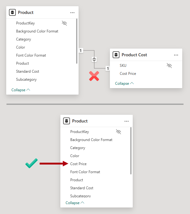
One-to-one cardinality allows you to relate two tables that each have a unique column. This type of relationship isn't common because it's considered a better practice to use Power Query to merge queries to produce a single model table. That way, you reduce the number of model tables and produce a more intuitive experience for report authors, who can find related fields in a single table.

Consider a scenario where there's a Product Cost table that contains the Cost Price column, which is sourced from a supplementary data store. Its SKU column contains the product stock-keeping unit (SKU). When a relationship is created to the Product table on the ProductKey column, a one-to-one relationship is established because both columns contain unique values.

In a second scenario, the modeler takes a different approach. They merge the Power Query queries together and add the Cost Price column to the Product query. They then disable the load of the Cost Price query. It results in only one product table.

Many-to-many cardinality allows you to configure complex relationships between model tables. It's useful when there isn't a column of unique values. For example, the Target table stores facts at product category level, yet the Product table stores products at product SKU level. While the ProductKey column stores the SKU, the Category column stores the category name, of which there are many duplicates. When you relate the Category column of the Product table to the Category column of the Target table, the cardinality must be set as Many-to-many. In this instance, it allows relating a dimension table to a fact table at a higher level or granularity.

Understand cross filter direction

A model relationship is defined with a cross filter direction. The direction determines how filters propagate. Where there's a "one" side, filters always propagate to the other side. Where there's a "many" side, it's possible to allow propagation to the other side too.

The possible cross filter options are dependent on the relationship cardinality type:

• One-to-many (or Many-to-one): Single or both
• One-to-one: Both
• Many-to-many: Single to either table, or both

Generally, it's a good practice to avoid or minimize cross filters in both directions. That's because it results in better query performance and usually produces an intuitive experience for report consumers.

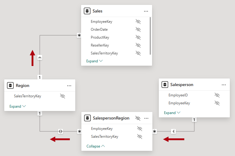
A valid reason to allow cross filtering of a one-to-many relationship in both directions is to enable many-to-many analysis between two dimension tables. Consider an example where salespeople are assigned to multiple regions, and conversely regions can have multiple salespeople assigned. To implement this design, your model needs a bridging table that associates salespeople and regions.

The following screenshot shows a model diagram that relates the Salesperson table to Sales table. The SalespersonRegion table, which is a bridging table, contains the EmployeeKey and SalesTerritoryKey columns, of which neither contains unique values. Notice how the filter propagation works:

1. Filters applied to the Salesperson table propagate to the SalespersonRegion table.
2. Filters applied to the SalespersonRegion table propagate to the Region table because cross filtering is supported in both directions.
3. Filters applied to the Region table propagate to the Sales table.

Active vs. inactive relationships

There can only be one active filter propagation path between two model tables. However, it's possible to introduce other relationship paths, though you must set these relationships as inactive. Inactive relationships can only be made active during the evaluation of a model calculation by using the USERELATIONSHIP DAX function.

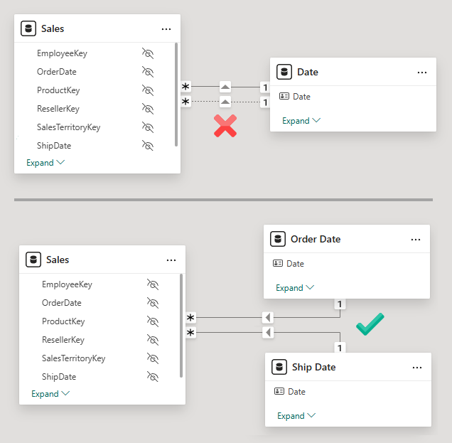
It's common enough that multiple relationships to a dimension table exist, which is known as a role-playing dimension. For example, consider that the Sales table has two date columns: OrderDate and ShipDate. However, if you relate both columns to the Date table, only one relationship can be active.

To allow filtering by either order date, ship date, or both at the same time, you need two date tables. By creating Order Date and Ship Date tables, each can have active relationships to the Sales table.

The following screenshot compares two model design scenarios. The first scenario shows a single date table with an active and inactive relationship. The second scenario shows two dates tables, each with active relationships. (Active relationships are represented by solid lines; inactive relationships are represented by dotted lines.)

Work with the model diagram

In the model diagram, relationships are represented by the lines that connect tables.

An easy way to create a relationship is to drag and drop columns between tables in the model diagram. An easy way to edit a relationship is to simply double-click it.

You can interpret the properties of a relationship by viewing it in the model diagram:

• The cardinality of a relationship is described by the "one" (1) or "many" (*) icons located at the ends of the relationship line.
• The cross filter direction of a relationship is described by the arrows located in the middle of the relationship line.
• An active relationship is a solid line; an inactive relationship is a dotted line.

To determine which columns are related, you can hover the cursor over the relationship to highlight the related columns.